Knowledge Distillation
May 4, 2018
This blog first appeared at Intel Devpost. Here is the link
Hinton, Geoffrey, et al. “Distilling the Knowledge in a Neural Network.” arXiv, 9 Mar. 2015, arxiv.org/abs/1503.02531v1.
Associated code can be found on Github.
Abstract
The problem we are facing right now is that we have built sophisticated models that can perform complex tasks, but the question is: how do we deploy such bulky models on our mobile devices for instant usage? Obviously, we can deploy our model to the cloud and call it whenever we need its service, but this would require a reliable internet connection and hence becomes a constraint in production. So what we need is a model that can run on our mobile devices.

So what’s the problem? We can train a small network that can run on the limited computational resources of our mobile device. But there is a problem with this approach. Small models can’t extract many complex features that can be handy in generating predictions unless you devise some elegant algorithm to do so. Though ensembles of small models give good results, unfortunately making predictions using a whole ensemble of models is cumbersome and may be too computationally expensive to allow deployment to a large number of users. In this case, we resort to either of these 2 techniques:
- Knowledge Distillation
- Model Compression
If you have developed a better solution or if I might have missed something, please mention it in the comments 🙂
In this blog, we will look at Knowledge Distillation. I will cover model compression in an upcoming blog.
Knowledge distillation is a simple way to improve the performance of deep learning models on mobile devices. In this process, we train a large and complex network or an ensemble model which can extract important features from the given data and can, therefore, produce better predictions. Then we train a small network with the help of the cumbersome model. This small network will be able to produce comparable results, and in some cases, it can even be made capable of replicating the results of the cumbersome network.
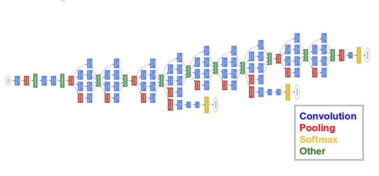
For example, since GoogLeNet is a very cumbersome (meaning deep and complex) network, its depth gives it the ability to extract complex features and its complexity gives it the power to remain accurate. But the model is heavy enough that one would surely need a large amount of memory and a powerful GPU to perform large and complex calculations. That’s why we need to transfer the knowledge learned by this model to a much smaller model which can easily be used on mobile devices.
About Cumbersome Models
Cumbersome models learn to discriminate between a large number of classes. The normal training objective is to maximize the average log probability of the correct answer, and it assigns probabilities to all the classes, with some classes given small probabilities with respect to others. The relative probabilities of incorrect answers tell us a lot about how this complex model tends to generalize. An image of a car, for example, may only have a very small chance of being mistaken for a truck, but that mistake is still many times more probable than mistaking it for a cat.
Note that the objective function should be chosen such that it generalizes well to new data. So it should be kept in mind while selecting an appropriate objective function that it shouldn’t be selected in such a way that it only optimizes well on training data.
Since these operations will be quite heavy for mobile devices during performance, to deal with this situation, we have to transfer the knowledge of the cumbersome model to a small model which can be easily exported to mobile devices. To achieve this, we can consider the cumbersome model as the Teacher Network and our new small model as the Student Network.
Teacher and Student
You can ‘distill’ the large and complex network into another much smaller network, and the smaller network does a reasonable job of approximating the original function learned by the deep network.

However, there is a catch: the distilled model (student) is trained to mimic the output of the larger network (teacher), instead of training it on the raw data directly. This has something to do with how the deeper network learns hierarchical abstractions of the features.
So how is this transfer of knowledge done?
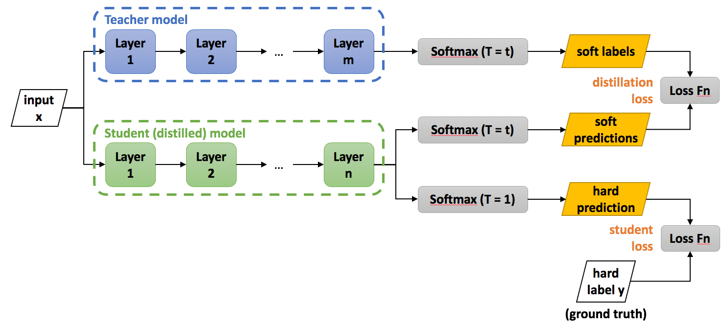
The transferring of the generalization ability from the cumbersome model to a small model can be done by using the class probabilities produced by the cumbersome model as “soft targets” for training the small model. For this transfer stage, we use the same training set or a separate “transfer” set as used for training the cumbersome model. When the cumbersome model is a large ensemble of simpler models, we can use the arithmetic or geometric mean of their individual predictive distributions as the soft targets. When the soft targets have high entropy, they provide much more information per training case than hard targets and much less variance in the gradient between training cases, so the small model can often be trained on much less data than the original cumbersome model while using a much higher learning rate.
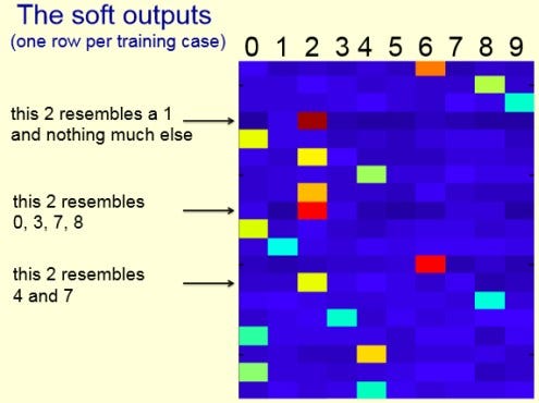
Much of the information about the learned function resides in the ratios of very small probabilities in the soft targets. This is valuable information that defines a rich similarity structure over the data (i.e., it says which 2’s look like 3’s and which look like 7’s, or which “golden retriever” looks like a “Labrador”) but it has very little influence on the cross-entropy cost function during the transfer stage because the probabilities are so close to zero.
Distillation
For distilling the learned knowledge, we use Logits (the inputs to the final softmax). Logits can be used for learning the small model, and this can be done by minimizing the squared difference between the logits produced by the cumbersome model and the logits produced by the small model. The equation below represents softmax with temperature.
\[P_t(a) = \frac{\exp(q_t(a)/\tau)}{\sum_{i=1}^n\exp(q_t(i)/\tau)}\]For high temperatures (\(\tau \rightarrow \infty\)), all actions have nearly the same probability, and at lower temperatures (\(\tau \rightarrow 0\)), the expected rewards affect the probability more. For low temperature, the probability of the action with the highest expected reward tends to 1.
In distillation, we raise the temperature of the final softmax until the cumbersome model produces a suitably soft set of targets. We then use the same high temperature when training the small model to match these soft targets.
Objective Function
The first objective function is the cross-entropy with the soft targets, and this cross-entropy is computed using the same high temperature in the softmax of the distilled model as was used for generating the soft targets from the cumbersome model.
The second objective function is the cross-entropy with the correct labels, and this is computed using exactly the same logits in softmax of the distilled model but at a temperature of 1.
Training ensembles of specialists
Training an ensemble of models is a very simple way to take advantage of parallel computation. But there is an objection that an ensemble requires too much computation at test time. However, this can be easily dealt with using the technique we are learning. And so “Distillation” can be used to deal with this issue.

Specialist Models
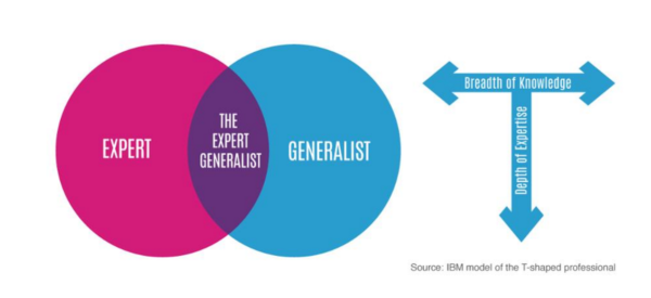
Specialist models and one generalist model make up our one cumbersome model. The Generalist Model is trained on all training data, and Specialist Models focus on different confusable subsets of the classes to reduce the total amount of computation required to learn an ensemble. The main problem with specialists is that they overfit very easily. But this overfitting may be prevented by using soft targets.
Reduce Overfitting in Specialist Models
To reduce overfitting and share the work of learning lower-level feature detectors, each specialist model is initialized with the weights of the generalist model. These weights are then slightly modified by training the specialist, with half its examples coming from its special subset, and half sampled at random from the remainder of the training set. After training, we can correct for the biased training set by incrementing the logit of the dustbin class by the log of the proportion by which the specialist class is oversampled.
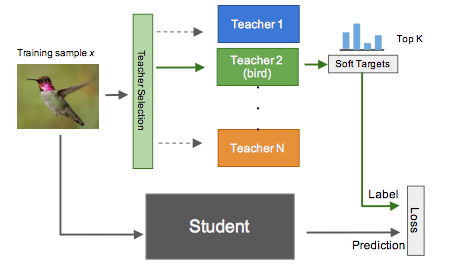
Assign classes to Specialists
We apply a clustering algorithm to the covariance matrix of the predictions of our generalist model so that a set of classes Sm that are often predicted together will be used as targets for one of our specialist models, m. So we apply K-means clustering to the columns of the covariance matrix to get our required clusters or classes.
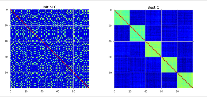
Covariance/Correlation clustering provides a method for clustering a set of objects into the optimum number of clusters without specifying that number in advance.
Performing inference
For each test case, we find the ‘n’ most probable classes according to the generalist model. Call this set of classes k.
We then take all the specialist models, m, whose special subset of confusable classes, Sm, has a non-empty intersection with k and call this the active set of specialists Ak (note that this set may be empty). We then find the full probability distribution q over all the classes that minimizes:
\[KL(p^g, q) + \sum_{m \epsilon A_k} KL(p^m, q)\]KL denotes the KL-divergence. \(p^m\), \(p^g\) denote the probability distribution of a specialist model or the generalist full model.
\[KL(p||q) = \sum_{i}p_i \log {p_i \over q_i}\]The distribution \(p^m\) is over all the specialist classes of \(m\) plus a single dustbin class, so when computing its \(KL\) divergence from the full \(q\) distribution, we sum all of the probabilities that the full \(q\) distribution assigns to all the classes in \(m\)’s dustbin.
Soft Targets as Regularizers
Soft Targets or labels predicted from a model contain more information than binary hard labels due to the fact that they encode similarity measures between the classes.
Incorrect labels tagged by the model describe co-label similarities, and these similarities should be evident in future stages of learning, even if the effect is diminished. For example, imagine training a deep neural net on a classification dataset of various dog breeds. In the initial few stages of learning, the model will not accurately distinguish between similar dog breeds such as a Belgian Shepherd versus a German Shepherd. This same effect, although not so exaggerated, should appear in later stages of training. If given an image of a German Shepherd, the model predicts the class German Shepherd with high accuracy, the next highest predicted dog should still be a Belgian Shepherd or a similar-looking dog. Over-fitting starts to occur when the majority of these co-label effects begin to disappear. By forcing the model to maintain these effects in the later stages of training, we reduce the amount of over-fitting. Though using soft targets as Regularizers is not considered very effective. Check out this blog by neptune.ai to get more ideas about different algorithms used for knowledge distillation.
Follow me on twitter @theujjwal9